
After completing this course, you will:
Understand how to design a culvert
Have reviewed Manning’s Equation and Hazen-William’s forumla, and how to use both to determine gravity flow
Have a tool to help make short work of a tedious task
INTRODUCTION
A stormwater “conveyance system” includes the drainage facilities and features, both natural and constructed, which collect,
contain and provide for the flow of surface and storm water from the highest points on the land down to a receiving water.
In the late 1800’s, Robert Manning came up with a formula for flow in systems that were working by gravity, that is pipes and
ditches that were not full or under pressure. In addition, the Hazen Williams formula was developed for flow in confined
systems.
This course contains a useful spreadsheet which implements both formulas into a convenient location for quick use. Download
Course Excel this spreadsheet by clicking on this link: Spreadsheet Download and save the file to your computer. You
will need this spreadsheet later in the course.
BASIC CIVIL ENGINEERING
CULVERT DESIGN 2
Gravity Flow (quick review)
Gravity flow through pipes not under pressure is usually determined using the Manning formula developed by Robert
Manning. Robert Manning was an engineer born in Wicklow, Ireland. He had a long career in Dublin and Belfast during the
latter half of the 1800’s. He is famous for hydraulic engineering and in textbooks for the “Manning Coefficient”, still in use to
describe water flow in open channels.
The most commonly used empirical equation to determine open channel flow is Manning’s Equation:
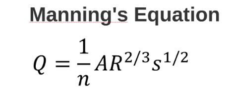
v = K/n R 2/3 S 1/2
v = Fluid Velocity (ft/s) or [m/s]
K = 1.486 (English); K = 1.00 [SI]
R = Hydraulic Radius (ft) or [m] = A/Pw
A = Cross-Sectional Area of Flow (ft2) or [m2]
Pw = Wetted Perimeter (ft) or [m]
S = Channel Slope
n = Manning’s Roughness Coefficient
The cross-sectional area to flow and wetted perimeter are related to the depth.
Pressure Flow
Flow through pipes under pressure is usually determined using the Hazen-Williams formula (An equation developed in 1902
by Gardner Williams and Allen Hazen to express flow relations in pressure conduits):
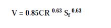
In this equation the roughness coefficient is C. The other factors are the same as the Manning Formula.
NOTE: The Hazen Williams formula is for a maximum internal velocity of 22 fps. If you ABSOLUTELY have to
exceed 22 fps use a friction loss calculation program based on the laminar/turbulent flow equations of
Darcy-Weisbach, a standard civil engineering calculation method. You would no longer be designing a system
that will work in the long run due to scour, but at least the flows and pressure you calculate will be closer to
what actually occurs in real life.
Typical roughness values
Values of C in Hazen-Williams formula, taken from Williams and Hazen’s book “Hydraulic Tables” and other authorities.
C = 145 : Asbestos-cement pipe.
C = 140 : Bitumen-lined steel pipes; smooth concrete pipe; smooth pipes of brass, glass or lead.
C = 130 : New coated cast iron pipe; small brass or copper pipe.
C = 125 : New uncoated cast iron pipe.
C = 120 : Smooth woodstave pipe.
C = 110 : Riveted steel pipe; vitrified pipe,
C = 100 : Brick sewers.
For old or encrusted pipes the value of C may be as low as 80 or less, depending on the actual condition.
Values of Manning’s “n” for Channels
n = .009 : straight channels of smooth planed boards.
n = .010 : neat cement plaster.
n = .012 : unplaned boards; sand and cement plaster.
n = .013 : steel trowelled concrete; metal flumes.
n = .014 : wooden troweled concrete.
n = .015 : ordinary brickwork or smooth masonry.
n = .020 : channels in fine gravel; rough set rubble; or earth in good condition.
n = .025 : canals and rivers in fair condition
n = .030 : canals and rivers in poor condition.
n = .035 : canals and rivers in bad condition, say with bed strewn with stones and detritus.
n = .040 : canals half full of vegetation.
n = .050 : canals two-thirds n = full of vegetation.
As the Manning formula is sometimes used for flow in pipes, the following table of values of “n” may be useful. The value of
V being found by the Manning formula on the “channels” side of the rule, this may be applied on the “pipes” side to find the
flow.
Values of Manning’s “n” for Pipes
n = .010: Asbestos-cement pipe
n = .011: Concrete pipe; very smooth.
n = .012: Clean coated cast iron pipe; woodstave pipe.
n = .013: Clean uncoated cast iron pipe.
n = .014: Vitrified sewer pipe; riveted steel pipe.
n = .015: Galvanized iron pipe.
n = .016: Concrete pipe with rough joints.
n = .021: Corrugated metal pipes.
Old or badly encrusted pipes will require higher values of “n” depending on the actual condition. In addition, the following
table may be useful (thousands of values of “n” have been computed, the internet is a great place to find the one you may be
looking for):
Material Manning (n) Hazen-Williams (C)
Plastic, copper 0.009 160
Concrete – Smooth 0.011 120
Concrete – Design 0.013 100
Corroded Cast Iron 0.020 60
Spreadsheet
The purpose of the spreadsheet is to provide one with a quick and easy way to develop a system of pipes to conduct fluids.
The spreadsheet solves either for gravity flow or submerged flow. The construction of a series of pipes is done by copying and
pasting example culverts, one after another into the spreadsheet. The end result will be a worksheet showing all the culverts –
interconnected, with drainage areas, required flow capacity, actual capacity, rims, inverts, slopes, lengths, velocity, depth to
hydraulic grade, etc., – everything needed by the draftsman and the reviewer to see how you came up with your design.
Begin
When you open the spreadsheet you will see line 21 of the “Calculations” worksheet. If you notice, there are four worksheets,
the first is “Calculations”, the second is “Forms”, the third is TOC, and the fourth is C. I will call this entire spreadsheet
Culvert Design 2 (CD2), the first worksheet I will call Calc, the second sheet Forms, the third TOC, and the fourth C.
At this time I think it is a good idea to “snoop around” a little bit. As indicated above, CD2 has four worksheets. If you click
on worksheet “Forms”, you will see the options available. If you want, the advanced student can add other options here. The ones available are Mannings culvert, and flume, and, to the right, Hazen Williams.
These blocks of the worksheet are copied onto the “Calculations” worksheet, then modified to model your situation.
If you click on “TOC” you will find a number of blocks set up to determine the time of concentration. There are a number of
factors of n on the right side of the worksheet – you may interpolate between them if necessary. If you fill in the actual lengths
that the water will run over grass or pavement and the slopes, etc. you can calculate quite closely the TOC for each area.
If you click on “c” you will find several blocks where you can calculate the coeffient of runoff for areas which are made up of
pervious and impervious surfaces. You can modify this easily to suit your purpose. The resultant C is a ratio, thus you can use
acres, hectares or any other value, not just square feet, for the area.
Now let’s go back to the “Calculations” worksheet.
The Calc worksheet has, at the top, some directions as a reminder of the basic things you can do with this spreadsheet — arrow
up to review them:
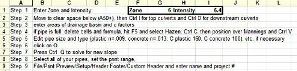
Step 1 directs you to cell G1 to enter the FDOT zone you are in (see below for the Florida Map showing our zones):
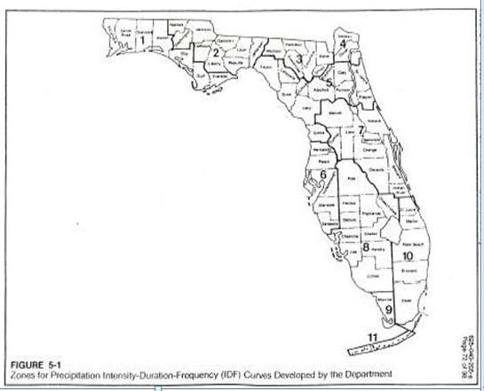
This number is not used in any calculations, it is only displayed on each sheet as a reminder of the Zone you are working in,
Cell I1 shows the intensity which will be used as a default for each culvert. Below is a graph for Zone 6.
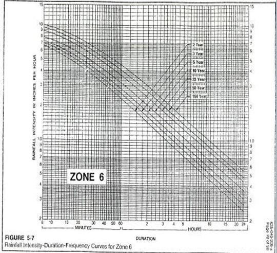
I have used 6.4 inches per hour as the average 15 minute TOC intensity value to get a rough idea of pipe sizes.
On to the spreadsheet!
When you open CD2 your cursor will be at A50. If for example, you have five culverts flowing by gravity, all conducting
water to the next in a series, your quickest way to get started is press “Ctrl-D” four times. Now you have (including the
original culvert) a total of five culverts, all interconnected. Next, scroll up to the first one (Area # 1) and begin modifying each
to model your system.
What you have done is copy a portion of Worksheet “Forms: over and over into the “Calculations” worksheet. This portion of
“Forms” could be either gravity flow or submerged, a pipe or a flume. The portion copied contains two parts, flow in from the
basin (on the left), and flow out (on the right).
Water Flowing In
The left side of the calculations should look something like this:
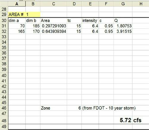
This portion of the sheet displays the calculations for the amount of water coming into the culvert (5.72 cfs in this example). If
you already know your flow you can just enter it in G48 (and delete the areas), if you do not, this portion of the worksheet is
set up to solve for it. Some aids to solving for this Q are shown on worksheets TOC and C.
Starting on the left, in columns A and B, are the dimensions of two areas. The first area flowing to this culvert is 70 feet by
185 feet. This amounts to 0.297 acres. If your areas are in square feet, enter the areas in cells A31 to A44 and a 1 in B31 to
B44. If your areas are already figured in acres, just enter the acres under C31 to C44 and delete the values A31 to A44, and B31 to B44.
Time of Concentration (tc)
If you want to figure a more accurate tc (Time of Concentration), click on the worksheet “TOC” and fill in the known values,
then copy the results to D31 to D44 on “Calc”. If you want to figure a more accurate c (coefficient of runoff), click on the
worksheet “C” and fill in the known values, then copy the results to F31 to F44. For this example we are designing a very flat
parking lot, thus the tc is set arbitrarily at 15 minutes, the c is 0.95, and the intensity is 6.4.
As we have two sub-areas coming to our inlet there are two areas shown. If there were a third you would click on A33 and
then “Ctrl-A”. This will add another sub-area for you to edit. If you have side flows coming in, you can add the flows at G33
to G44.
Now we should know pretty much how much flow needs to be handled by this culvert.
Quantity the Pipe Can Handle
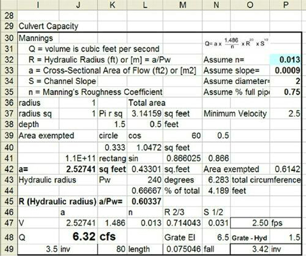
This is how the right half looks:
Some of the things this will tell you are:
P32 the Mannings “n” you select (see above for examples of n).
P33 the slope of the culvert, this is usually calculated and not touched, unless you have a specific slope you need to hold (for example if the pipe comes out of the ground).
P34 the pipe diameter, this is usually input as an estimated pipe size.
P35 the depth of water in the pipe, this can be any number 0 to 1, but usually is .75.
P37 minimum velocity, this is usually 2.5 but can be set to any number.
N48 Upstream grate elevation
K49 Length of your pipe
I49 and O49 Upstream and downstream inverts of pipe, usually the upstream invert is set only for the initial
pipe, it is solved for in the downstream pipes (with the exception of pipes which come out of the ground – these
need to be addressed seperately).
Numbers displayed for information only:
J36 the radius of the pipe
L37 area of full pipe
J42 area of partially full pipe
L45 Hydraulic radius
O47 Velocity in pipe
J48 Quantity pipe will flow
O48 The depth from the grate to the hydraulic gradient in the upstream end.
M49 The fall in the pipe (ft).
The default numbers need to be changed to match your situation:
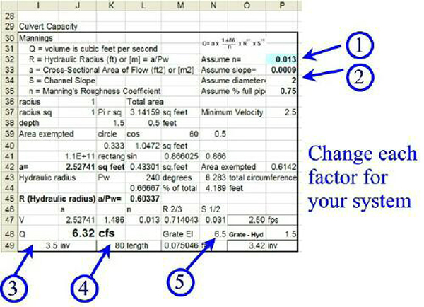
The five areas shown are the “usual suspects” which need attention. All cells are available for change, but do not: unless you
wish to be responsible. The obvious ones are the size, type, invert, length, and grate elevation. Another is cell O47 the
minimum velocity, if you desire something other than 2.5, change it here.
Next, the fun part:
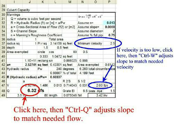
Previously you found your required Q, and have input your initial culvert guess, now go to J48 and click “Ctrl-Q” as shown
above. Your culvert is designed!
Now check it out. Is the velocity OK?– if it is too low, go to O47, click “Ctrl-W” and it will be adjusted. If it is too high, go to
P34 and put in a larger pipe, then go back to J48 and click “Ctrl-Q” again. You can also check out how fast you are “using up”
your available fall, and adjust if necessary.
That is all for the first culvert. Now go onto each of the four culverts you added below this. Make sure that the culverts do not
come out of the ground. If the invert of the downstream end of any pipe is not deep enough, impose a manditory slope in the
appropriate cell to insure cover. When you have tinkered enough, follow the directions for Step 8 (cell A8). Select all of your
pipes, click on File/Print Area/Set Print Area to insure that you get all the pipes you have designed. Next, the directions in
Step 9 (cell 9) helps you to label your project. Last, Print it!
Side Branches
Not all systems are quite that easy. Let us imagine we have the system above (A1 to A5) and a parallel run of two culverts
B1and B2 in another series that dump into your third culvert (let’s call that one A3).
STEP 1:
After the last culvert of the first series is entered, go to the bottom of the A column as if you were going to add another culvert (A134 in our example) and instead of “Ctrl-D”, you press “Ctrl-I”. You will add culvert B1 with no upstream culverts. Then
press “Ctrl-D” to add B2. So far so good, just modify them to match your system. Now they have to be tied in. B2 will show a
volume – let us say 10 CFS. This flow needs to be added to A3. First you write down the cell where the Q shows 10 cfs (G174
for example). Then go to the culvert that has to handle the additional flow. Scroll to column G where you have designed
culvert A3 (G77 for example) and enter “+G174”. This will input the correct flow (even if you make changes later). (Note,
don’t forget that this pipe and all downstream pipes need to be solved for if you make this change).
STEP 2:
We need to check our inverts next. The upstream invert for A3 (cell I91 in our example) needs to be lower than the
downstream invert for side branch B2 (cell O175 in our example). If it is not, in cell I91 enter “+O175”. This will insure that
the inverts will be maintained correctly.
Sanitary Conflicts
With many systems the storm sewers and the sanitary sewers try to use the same space. Lets imagine that a sanitary sewer
crosses the storm 25 feet down from the beginning of the first culvert. In cell K49 all you do is enter 25 and read your invert in
cell O49. This can be entered in row 50 if you wanted to keep a record of it (I have at times entered the formulas from row 49
into row 50 to keep a permanent record: make sure that you enter the proper formula in M50, this is the length in K50 times
the slope in P33). Do not forget to put back the true culvert length before proceeding if you have chnged it temporarily!
Changes
If you have to add another culvert (put two where there was one before — A3 for example needs to be replaced with two
culverts), just select the rows for the culvert below (A4), click Insert/Rows, then select the top left of the open space and
“Ctrl-D” to enter the new culvert. If a culvert is to be removed, select it and delete the rows.
Summary
Entering a series of culverts is easy, a series of “Ctrl-D” for each culvert. Then “Ctrl-I” to start a side branch and “Ctrl-D” for
each downstream from that; another “Ctrl-I” for another side branch, etc. until you have entered all of your culverts. The
default dimensions then are changed to match your system and the culverts are matched to your flows!
Other Options
Submerged pipe.
If, for example, your last pipe was submerged as it went into a pond, Mannings formula would not be appropriate. I
recommend that you solve the project as usual, then follow the following procedure.
In the “Culvert Capacity” portion of the spreadsheet for the culvert that is submerged, select all of the cells:
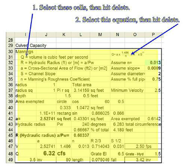
In the above example, select I30, then holding the Shift key, select cell P49. Then hit Delete to erase the contents. The formula
will remain, so you will have to select it and delete it as well.
Then select cell I30 again and press F5. Select “Hazen2” for a downsteam pipe. Press “Ok”. Then “Ctrl-C”. Click on the
Calculations tab. Then “Ctrl-V” to paste. Next select the Q as usual (you may have to click twice) and “Ctrl-Q” to solve for
the flow you need. Your velocity, pipe size, type, and all have to be checked to insure that you have the system you think you
do! The pipe inverts have been calculated for the hydraulic slope, but in reality they do not matter, I keep them so that debris
will fall out though,
Flume
If your end is a flume, the capacity of the flume can be modeled just like the submerged pipe. Delete the cell contents and
instead of selecting “Hazen2”, select “Flume”. After you paste the flume in place, enter the width and height, along with the
top elevation, length, and bottom elevations and your capacity will be displayed.
Final Notes
As with any spreadsheet, the change in any cell may affect the result. If you have any doubt, click on the cell to view the
contents before entering a number. If it is a formula, then be careful that you do not affect the results adversely.
None of the cells are protected, thus you can change anything in the spreadsheet.
Have fun!
CONCLUSION
The Manning and the Hazen-Williams formulas are very complicated, but the spreadsheet included in this course tames them.
With the entry of your specific areas drained to each culvert, and a few simple parameters for that culvert, with a touch of a
button you can design any given culvert. You can design a small project in a matter of a couple of hours.